Exercise 2 - ROS Development and Kinematics | Farfetch’d Robotics CMPUT 412 Website

Part 1 - ROS basics

ROS Concepts

Node: named modular computation process.
Topic: named message bus that routes messages that nodes can publish and subscribe to.
Service: named pair of request message from a client node and reply message from the providing node.
Message: typed data structure used for internode communication.
Bag: message data format

For this first section, we’ll be referencing code mostly in the heartbeat-ros workspace

Heartbeat ros package

We kicked things off by reading about ROS’s general publisher-subscriber model. To extend on the tutorial, we made a small package which simply sent a log message every ~50s. The publisher node publishes a custom message. The subscriber node then receives the message and prints it with loglevel INFO

To avoid hard coding the robot’s name, while still using topic names from root, we used an odd method to get the hostname by launching a subprocess. This works and technically is the most correct way to find a hostname, though we used the launch-file’s arg approach to pass in the hostname at runtime for all of the later packages

Camera modification

Next up was learning how to interact with pre-made topics on the duckiebot. We created a single node publishing 2 topics and subscribing to a different two.

To print the image size, we subscribed to camera_info and set a callback to print out a loglevel INFO message about the image’s dimensions. The callback also then republishes the string of the image dimensions to a topic called published_image_info.

On a tip from Justin, who mentioned it may be useful in future labs to remove color from the camera’s image, we attempted to republish a monochrome version of the image from the duckiebot’s camera. Doing this was simply a task for opencv. The camera callback reads in the raw image into a cv2 buffer, decodes it into cv2’s intermediary representation, applies a COLOR_BRG2GRAY filter, re-encodes it and published it to a topic called published_compressed.

So far we’ve only been mentioning the basename of the topic we’re publishing, and that’s since we didn’t actually publish to any of these topics. For this package, we tried to keep all our remapping in the camera.launch file. Our actually source code publishes to topics like ~published_image_info, though that’s just a descriptive placeholder for us to then remap in the launch file. The actual topics we published to were ~/camera_info and ~/compressed. The same method was used for the subscriber paths, taking advantage of the veh argument at runtime to determine the duckiebot’s name.

Keeping all the remapping in the launch file was helpful when we were still learning how to use name spacing properly. Quickly modifying the paths based on rqt_graph was easier when our launch file was dealing with all the paths, instead of having to constantly modify source code.

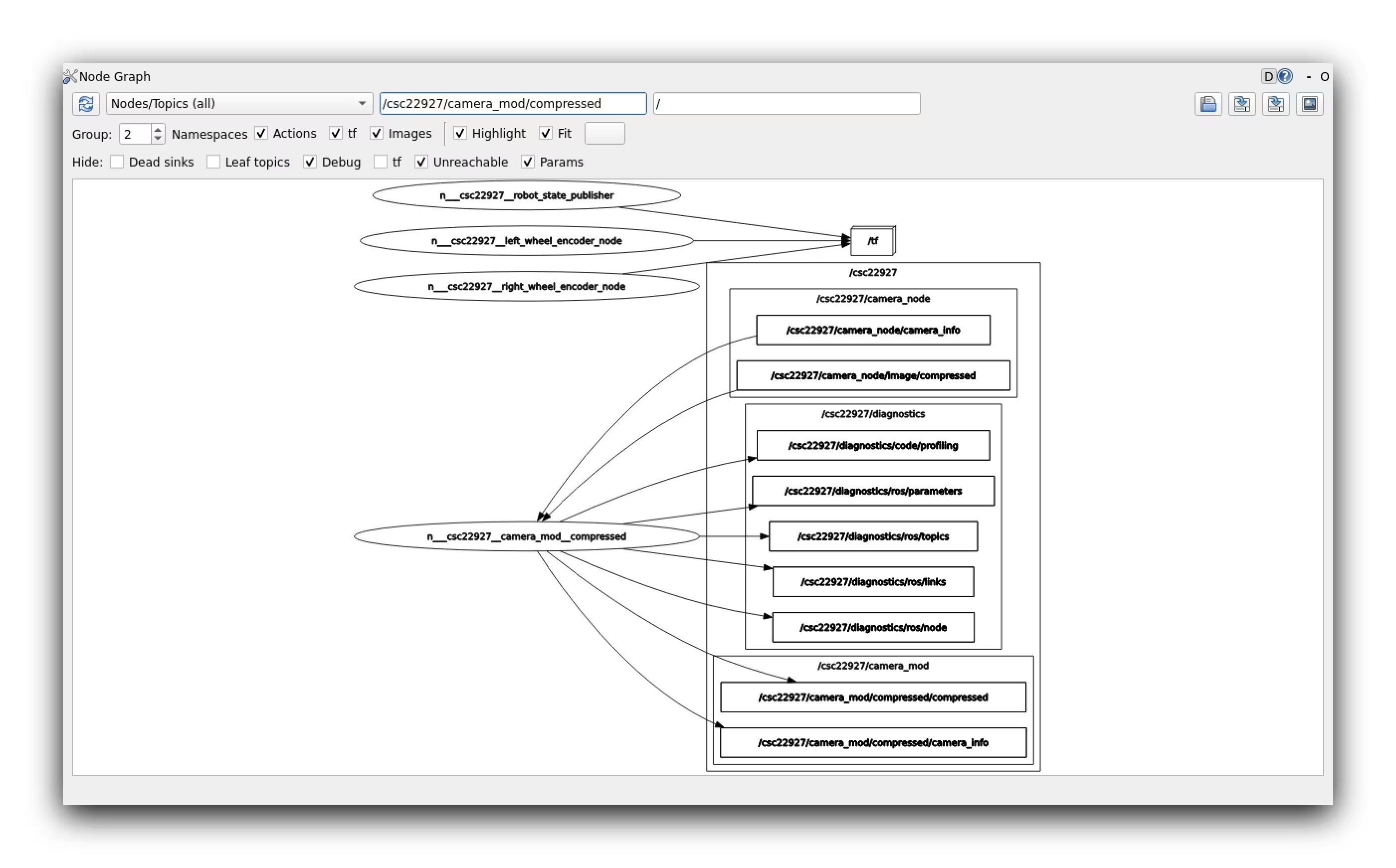
Here’s a screenshot of the node in rqt_graph:

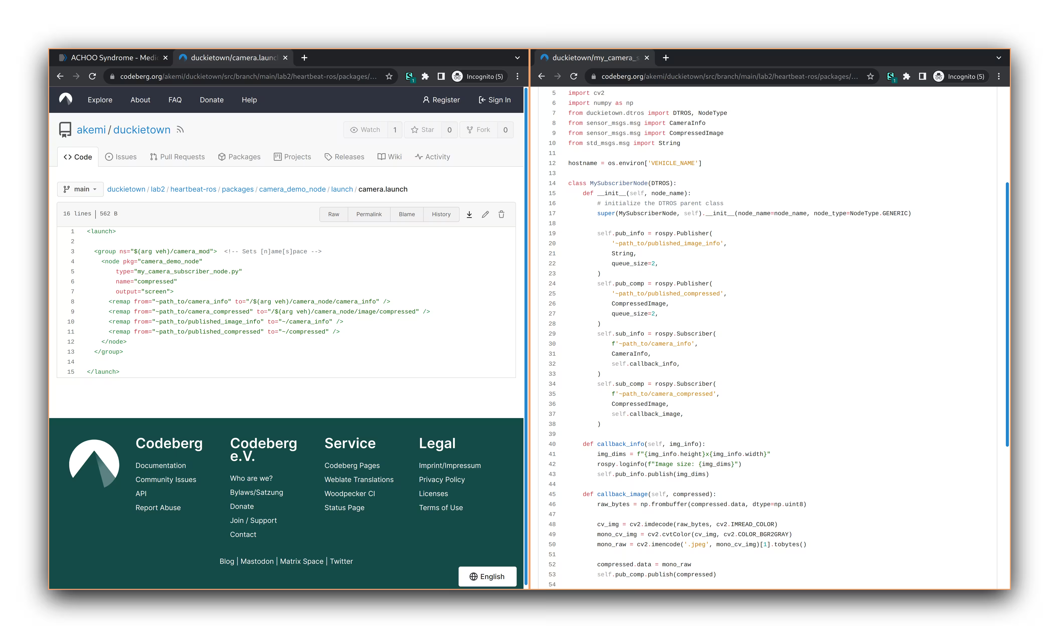
Custom camera node in rqt_graph. It publishes two outgoing topics

Notice how we used the word compressed as the basename of our published modified image’s topic name. While it usually doesn’t matter how topics are named, in this case it was very important our topic name ended with compressed. rqt_image_view is hardcoded to only consider topics ending with compressed, so publishing the same image to a topic called modified_image would fail to show up in rqt_image_view! Thanks to our classmate KarlHanEdn for discovering this and posting it on the discord

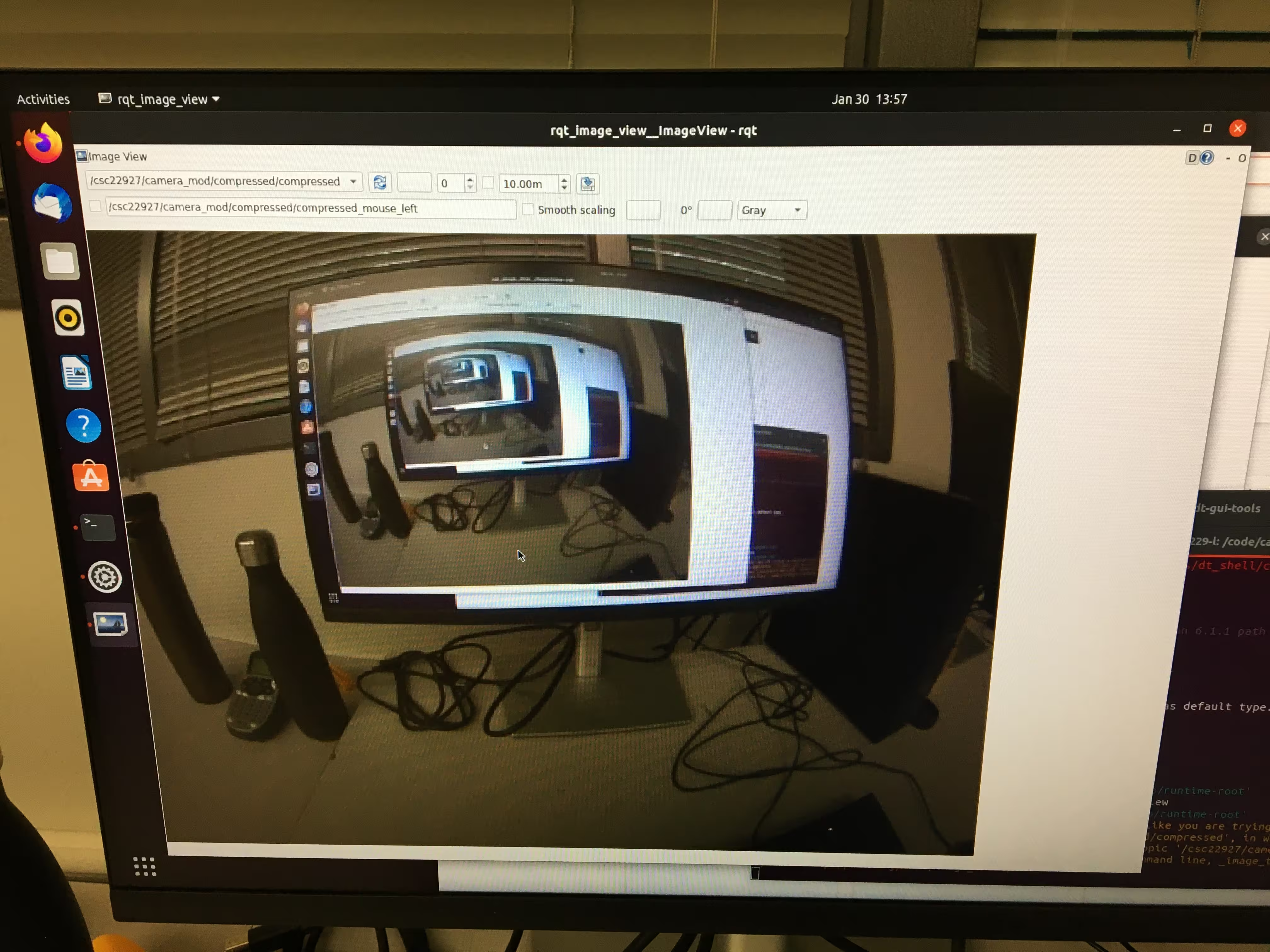
Here’s a screenshot of our modified topic being published (this one isn’t black and white):

Picture of screen with rqt_image_view streaming our topic

You can see the source code here, though the assignment asks for a picture of the source code… so here’s a picture of where the link leads:

Screenshot of 2 Chromium windows displaying source code

Robot Kinematics

What is the relation between your initial robot frame and world frame? How do you transform between them? How do you convert the location and theta at the initial robot frame to the world frame?

The robot frame is always centered on the robot, so it is given by

\[ \mathbf{\xi}_R = \begin{bmatrix} x_R \\ y_R \\ \theta \end{bmatrix} = \begin{bmatrix} 0 \\ 0 \\ \frac{\pi}{2}\end{bmatrix} \]

The initial world frame is given by \[ \mathbf{\xi}_I = \begin{bmatrix}x_I \\y_I \\\theta\end{bmatrix} = \begin{bmatrix}0.32 \\0.32 \\\frac{\pi}{2}\end{bmatrix}\]

To transform the initial world frame to the robot frame is trivial, keep the angle $\theta$ the same, and $x_R = 0$ and $y_R = 0$. This is equivalent to this matrix multiplication:

\[\mathbf{\xi}_R = \begin{bmatrix}0 & 0 & 0 \\0 & 0 & 0 \\0 & 0 & 1\end{bmatrix}\mathbf{\xi}_I\]

To get the initial world frame from the initial robot frame, we keep the angle $\theta$ the same, and set $x_I = 0.32$ and $y_I = 0.32$. This is equivalent to this matrix multiplication:

\[\mathbf{\xi}_I = \begin{bmatrix}1 & 0 & 0.32 \\0 & 1 & 0.32 \\0 & 0 & 1\end{bmatrix}\mathbf{\xi}_R\]

We used the following matrix multiplication to transform between the two:

\[\mathbf{\dot{\xi}}_I = \mathbf{R}^{-1}\mathbf{\dot{\xi}}_R\] with \[\mathbf{R}^{-1}(\theta) = \begin{bmatrix}\cos(\theta) & -\sin(\theta) & 0 \\\\\sin(\theta) & \cos(\theta) & 0 \\\\0 & 0 & 1\end{bmatrix}\]

Then we can update the world frame by integrating the above changes in world frame

\[\mathbf{\xi}_I = \mathbf{\xi}_I + \mathbf{\dot{\xi}}_I\]

We also must apply the modulo of $2\pi$ to the angle $\theta$ to keep it between $0$ and $2\pi$.

We note that the equation for getting the change in robot frame is given by

\[\mathbf{\dot{\xi}}_R = \begin{bmatrix} \frac{d_r + d_l}{2l} \\ 0 \\ \frac{d_r - d_l}{2l} \end{bmatrix}\]

where $d_r$ and $d_l$ are the integrated displacement traveled by the right and left wheels and $l$ is the distance between the wheels and the center of the rotation.

To get the integrated displacements $d_r$ and $d_l$, we use the wheel encoder ticks formula:

\[\Delta \text{ticks} = \text{ticks}_t - \text{ticks}_{t-1} \]

\[d_r = 2\pi \cdot r \cdot \frac{\Delta \text{ticks}}{\text{resolution}}\]

where $r = 0.025$ is the radius of the Duckiebot wheel and $\text{resolution} = 135$ is the number of ticks in one rotation of the wheel.

How did you estimate/track the angles your DuckieBot has traveled?

To update the angle $\theta$ that our DuckieBot has traveled, we used the matrix multiplication above, which breaks down to the following equations for angle:

\[\theta = \theta + \dot{\theta}\] where \[\dot{\theta} = \frac{d_r - d_l}{2l}\]

Can you explain why there is a difference between actual and desired location?

There are small errors that are mostly due to slippage and momentum. Since we do dead reckoning, as the DuckieBot moves more the small errors compound. We note that errors in the angle tend to drastically affect the bot’s x, y position due to the trigonometric functions used in matrix. This causes the Duckiebot’s desired location to drastically different from the actual location.

Which topic(s) did you use to make the robot move? How did you figure out the topic that could make the motor move?

For our first wheel-moving demo we published into the /$(arg veh)/wheels_driver_node/wheels_cmd topic. We found this topic with a mix of rostopic list, rostopic info, and rostopic echo while using the joystick to figure out which topics published what. Just as with the camera node, we took advantage of remapping in the launch file with arg to let this run on different duckiebots. We only used the wheel velocities on this topic’s message (WheelsCmdStamped) to guide it forward and negative velocities to guide it backwards. However we mostly scrapped this code, since the node didn’t bother localizing itself. This’d mean if one of the motors spins slower the other, the bot would be completely off. It even makes it harder to guarantee we traveled 1.25m, since the two wheels had different distances traveled. While there is a pre-built duckietown topic which gives pose, we instead opted to make a small modification out our dead reckoning code from section 2 to record the video linked below.

The above video shows our duckiebot going forward then back. We were using a pretty high speed for this one, hence the little jump it does when starting to reverse. We also hypothesized that part of the problem here lies in how we immediately go in reverse gear, instead of slowing down to a stop, then going in reverse. We use this slowing-down idea for section 2, particularly with our turning logic.

We tried several speeds and came to an amusing conclusion. Using very slow speeds ~0.3 and very high speeds like 1.0 resulted in about a 10-20cm difference between the starting and final position. However using intermediary speeds like 0.7, which we thought would do best, actually performed the worst, with and about 20-40cm difference between the starting and ending positions. For the slow case, the movement are accurate just since the duckiebot doesn’t introduce nearly as much noise from slippage and momentum. However for high speeds, it seems the slippage and momentum actually balances out! While the duckiebot will drift longer from momentum, it will also read more traveled distance when its wheels quickly slip. We were quite surprised about this, since we expected the higher the speed the higher the noise, though our 3 empirical runs simply don’t support that conclusion

Rotation task

The rotation task was pretty much identical to the driving forward task. We used the same publisher (/$(arg veh)/wheels_driver_node/wheels_cmd), just now we’d make one of the wheels go in a negative velocity, while the other is positive. To figure out our turn angle, we used a pretty simple formula to measure the difference in angle. When we forgot the modulo, our bot sometimes continued spinning forever. As you’ll notice in the code, there’re no guarantees that bot will nail its turn on the first try. Especially when we used high velocity turns, the bot would often miss the target angle and make a complete rotation once more before aligning up correctly. While this seems inefficient, when we tried to make it turn in the closest direction, the slippage this back-forth adjustment introduced so much noise, the duckiebot’s angle ended up being absurdly far off at high speeds.

In general, slow speeds worked much better for turning. Just look at this supposed -90 degree turn at max velocity on both wheels.

When we tested in the simulator, we used a turning velocity of 0.3 and that worked perfectly. It was going to work nicely in practice too… until we actually tried it. Turns out, the duckiebot is so heavy, it cannot complete a 90deg turn at any velocity under 0.6. On our second duckiebot, it sometimes managed with 0.5, though both just came to a halt when we tried 0.4. This requirement for high-speed turns persisted as the largest problem in getting demo right in section 2.

Graceful shutdown

This wasn’t mentioned in the previous sections, despite being used in the driving one, though we used a rospy.on_shutdown() hook to make sure our nodes would shutdown correctly. This method takes in a callback function which is called when rospy is shutdown. Notably for the driving nodes, it was very important that we stop the wheels before the node exits, otherwise it’d endlessly spin. However, that just lead us to write a small script to stop the wheels

rostopic pub -f my_msg.yml /path/to/topic msg/type
# Actually used example
rostopic pub -f stopstop /csc22927/wheels_driver_node/wheels_cmd duckietown_msg/WheelsCmdStamped

Since the duckiebots occasionally still crash the script without calling shutdown hooks, this method still ended up being a useful emergency stop for us

Section 2 - Driving robot through stages

General architecture

For section 2, we used 3 nodes across 2 packages. You can view the code here.

The odometry package includes two nodes. The first node called odometry_publisher_node does our kinematics and localization calculations. Each wheel is represented by its own dictionary. We mostly do calculations off the /{hostname}/{left,right}_wheel_encoder_node/ticks topic, which publishes the number of total ticks a wheel has accumulated. According to the documentation, this is 135 per full rotation. Since each wheel likely has a non-zero amount of ticks when our node starts up, we start by overwriting the number of wheel ticks taken on the first callback, then relative changes can be calculated properly

The other package contains the LED node, which provides a service interface. This is called from the odometry_driver_node, which acts as our central “state” node

LED service

We first implemented the LED node using the standard publisher-subscriber model that’s usually performed in ROS. This was pretty simple, we just construct an LEDPattern message then publish it to the /{hostname}/led_emitter_node/led_pattern topic. This worked pretty well, though we did notice in slow-motion footage that the front LEDs end up switching noticeably faster than the back LEDs. We didn’t notice any difference with our human eyes. This approach also sometimes just went wonky. Roughly 1/4 runs ended up with a heterochromic duckiebot, at least at one of the states.

In retrospect, we realized the problem is likely since we only publish once. We should have taken advantage of the service-wrapper to set a message on our led publisher node, then just have it continuously publish whatever the current message is at a few Hz. That may have turned out duckiebot back to solid-colors if the first message got poorly read or something.

Now with the publisher-subscriber model in place, we needed to introduce a service interface to this node. This took 1 line, though about an hour of playing around with it since the official tutorial was a bit confusing about mixing the two models together. In the end, it looks very similar to a subscriber from the server-side and a publisher from the client-side, though of course the code is blocking. For our specific case, the code works just as well with the publisher-subscriber model, though this community forum post seems generally in support of a service for how we’re using it.

We tested our service by having the node call its own service in a while loop while alterating colors. The bot ended up looking like a Christmas tree, though we noticed when the node shutdown it’d leave the last color running. To address this, we read up on shutdown hooks and set one so that when the led controller node shuts down, it turns off its lights.

On an amusing note, the LEDPattern message is written in rgba. Usually the a means transparency, so Akemi guessed it must mean the brightness in our context. However it turns out a lower a value gives “transparency” in the sense of white saturation, so we’d get very pale colors. This leaves us wondering if we can adjust the brightness beyond on-off, though we didn’t figure that out of this assignment.

Movement

Getting the movement right took by far the most effort in this lab. Before we continue, look at how well it ended up!

Except, that was from the wrong starting position :sob:.

We weren’t able to get such a lucky run from the correct starting position, though here’s our best recording:

Something seemed to keep tripping it up on that specific starting tile, since it worked so much better from the middle.

Before even trying to move the bot, Steven Tang decided to make a simulator so that we could develop the code at home without the duckiebot. He pretty much took the duckietown wheel driver node then added tick publishers for each wheel. He then added a run function which simulated the bot actually moving, while updating its wheel velocities based on what our odometry node is publishing to the /{hostname}/wheels_driver_node/wheels_cmd.

This is really cool, since it let us work out all the math and dead-reckoning ahead of time. It was working in the simulator perfectly. Then we put it on the duckietbot and it didn’t even move…

As mentioned previously, we found out the duckiebot doesn’t have enough power to turn without setting the wheel velocity magnitude to at least 0.6, at which point so much noise is added, the calculations done in the simulator ended up completely off.

We still retained the localization-based turning from before though. Instead of telling the duckiebot to turn -90deg at the start, we told it to turn to 0deg in the world frame.

In the end, our code ended up being very procedural. For each state, we have a different function. In general they start off by using a service request to change the LED color, then either move or just wait until the state is considered over. As usually goes for procedural code like this, manual tuning becomes really important. We needed to tune a lot, which was an extremely slow process with the provided duckietown docker container. Every time we changed a single parameter like the speed, the entire catkin build system would rerun, which took about 2mins.

To accelerate this, we ended up with a very hacky parameters file. This json effectively stores global variables for the workspace. Nodes read this file in directly and adjust their instance parameters. The genius behind this is how the Dockerfile doesn’t have to rebuild the entire workspace, it only needs to copy over the updated param.json file, which reduced the build time to just a few seconds. We do know that ROS actually has a parameters system built in, which would allow modifying parameters at runtime too, though this method was quicker and easier for this lab. We’ll be looking to use the native ROS version in the upcoming labs, since the build time is unlikely to improve.

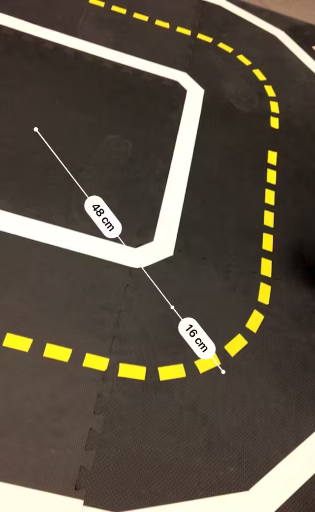
Our final video above is the same one from the start of this section. The final distance was 64cm when measured by AR-ruler. About 62cm when measured by a prehistoric 90cm-stick:

64cm measured distance in an AR-ruler screenshot of an iPhone

Putting it all together

For the video above, we recorded this bag. The video below, shows us playing it back on a local rosmaster and see the messages being sent live with rostopic echo.

and plotted it with matplotlib in this ipython-notebook, with the resulting image here:

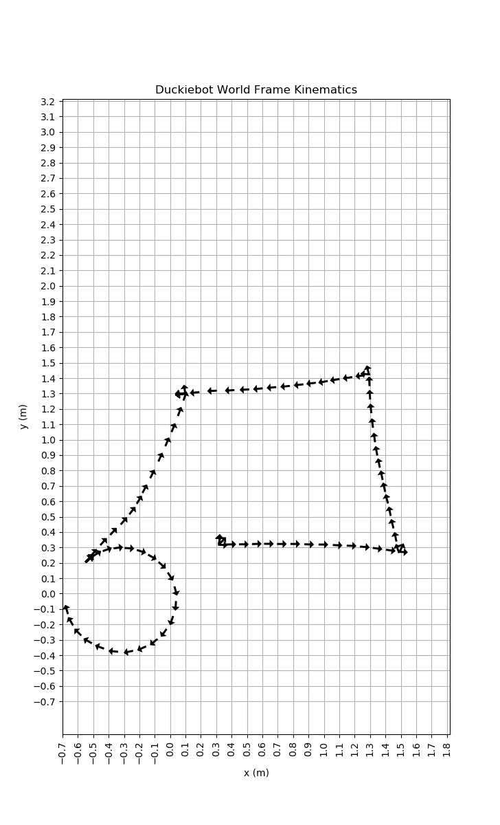
A quiver plot (end-to-end arrows) of the robot traveling in a square

This plot is showing what the duckiebot thinks it’s doing, which looking at the video clearly doesn’t align with what’s actually taking place. A quiver-plot is nice, since it gives us a pretty good idea of what the pose is. Notably, unlike scatter-plots, we can see the duckiebot turning on the spot in the 4 corners. We can also see the duckiebot go backwards from the top left corner down, just like we coded it up to do.

The initial turn, which in reality was the worst, looks as if it was nailed spot on. The duckiebot does pick up the slight drift is has when going in a straight line, which matches the results we saw in our forward-backward test from section 1.

We found it amusing how far off the results for our circle were though. In the quiver-plot, the duckiebot completely most of a perfect circle. In reality, it did about 1.5 circles in an ellipse. This was likely a mix of slippage, the wheel’s wobble, and the angle of the wheel on the duckiebot, which was certainly not perfectly parallel with the sides. To test out how bad it is, we modified our program to make the duckies go in an endless circle and launched it on both our duckiebots.

Even in that short clip, the two robots clearly had their circles change the amount they overlap from the start to the end, so there’s actually quite a bit of noise during the turn. On Tuesday Feb 6th’s lecture, we also learned how turning is disastrously more noisy than going in the straight line, so the quiver-plot’s disconnection from reality makes sense.